

Core idea. Portfolio concentration is not the number of open tickets. It is the amount of account risk that can be hurt by the same underlying event.
A retail FX platform can make a concentrated portfolio look diversified. EUR/USD, GBP/USD, AUD/USD, and USD/JPY appear as four separate symbols, with four separate charts, four stop-loss orders, and perhaps four different entry stories. Yet a trader who is long the first three and short USD/JPY is expressing essentially the same directional thesis four times: a weaker U.S. dollar.
That distinction is the heart of portfolio concentration. Pair count describes operational activity; concentration describes shared vulnerability. If one U.S. inflation release, Federal Reserve surprise, liquidity shock, or broad risk-off move can damage several positions together, those positions belong to the same risk conversation—even if their technical setups were identified independently.
This matters because leverage makes hidden overlap expensive. The CFTC warns that margin and leverage amplify both gains and losses in retail forex. Meanwhile, the BIS reported average global FX turnover of roughly $9.5 trillion per day in April 2025 and noted that the ten most-traded pairs all involved the U.S. dollar. A vast market and many tradable pairs do not automatically create independent bets. The dollar's central role can make portfolios look broader than they truly are.
Diversification Is About Independent Failure Paths
The useful question is not, “How many trades do I have?” It is, “How many different things must go wrong for all of these trades to lose?” A diversified portfolio has multiple failure paths. A concentrated portfolio has one dominant failure path wearing several ticker symbols.
Suppose one trade depends on U.S. dollar weakness, another on a risk-on rally, another on falling volatility, and a fourth on a range-reversion edge during the Asian session. Those positions may genuinely diversify one another if their loss mechanisms are different. By contrast, four breakout trades opened during London, all short USD and all dependent on continued trend expansion, combine currency, direction, session, regime, and strategy-family concentration.
Reality check. Different pairs are not necessarily different bets. Different entries are not necessarily different edges. Different stop distances are not necessarily different risks.
The six layers of FX concentration
| Layer | What is concentrated | Typical hidden link | Question to ask |
|---|---|---|---|
| Currency | Net long/short exposure | USD appears in several pairs | What is the portfolio's currency vector? |
| Macro driver | Sensitivity to the same catalyst | Rates, inflation, growth, risk sentiment | What event could move all positions together? |
| Strategy | Shared entry/exit logic | Every position is a trend breakout | Do the trades fail under the same regime? |
| Time | Positions opened in one window | London impulse or news burst | Is timing creating one clustered bet? |
| Volatility | Dependence on expansion or compression | Stops fail together when volatility jumps | What happens if volatility changes state? |
| Operations | Broker, platform, and execution dependency | One venue or one liquidity condition | Can one operational failure hit everything? |
Translate Every Pair into Its Currency Exposure Vector
Every spot FX position contains two legs. Buying EUR/USD means long EUR and short USD. Selling USD/JPY means short USD and long JPY. That sounds elementary, but many traders stop at the pair label and never aggregate the legs across the account.
The first professional upgrade is therefore a currency exposure vector: sum the directional risk assigned to each currency across every open position. Risk can be expressed as a percentage of equity, dollars at the initial stop, or standardized R-units. For a pre-trade decision, initial risk is usually the clearest common denominator.
| Position | Risk | Long leg | Short leg | Dominant shared thesis |
|---|---|---|---|---|
| Long EUR/USD | 0.50% | +0.50% EUR | −0.50% USD | USD weakness |
| Long GBP/USD | 0.50% | +0.50% GBP | −0.50% USD | USD weakness |
| Long AUD/USD | 0.50% | +0.50% AUD | −0.50% USD | USD weakness / risk-on |
| Short USD/JPY | 0.50% | +0.50% JPY | −0.50% USD | USD weakness / lower U.S. yields |
| Portfolio total | 2.00% gross | +0.50% each non-USD | −2.00% USD | One dominant short-USD cluster |
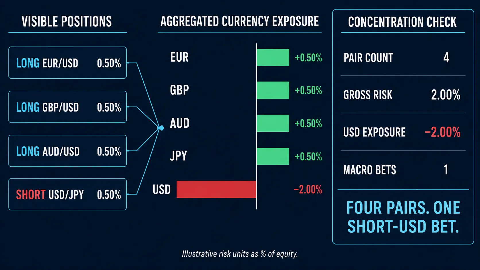
This vector is not a forecast of profit or loss; it is a map of directional dependence. Crosses can complicate the map but do not invalidate it. Long EUR/GBP and long GBP/JPY may partly offset GBP exposure while leaving EUR and JPY exposures intact. The aggregation step makes that visible before the account learns it through a correlated loss.
Correlation Changes the Size of the Bet
Currency vectors reveal directional overlap, but they do not fully describe joint behavior. Two positions can share USD exposure and still move with different intensity because their secondary currencies, sessions, catalysts, and volatilities differ. Correlation is the next layer.
For a set of positions with risk weights w and a correlation matrix C, a simple correlation-adjusted portfolio-risk proxy is:
Formula. Correlation-adjusted risk = √(wᵀ C w).This is a planning approximation, not a guaranteed loss bound.
Consider four positions risking 0.50% each. If their losses were independent, the risk proxy would be 1.00%. At an average correlation of 0.25, it rises to about 1.32%. At 0.60 it reaches about 1.67%; at perfect correlation it reaches the full 2.00% gross risk. The stop-loss amounts did not change. The portfolio geometry did.
Correlation is conditional, not permanent
A single 90-day correlation number is useful but incomplete. FX relationships vary with monetary-policy divergence, risk sentiment, commodity cycles, liquidity, and the release calendar. Correlation can also be asymmetric: positions may behave loosely together in ordinary conditions but become tightly linked during stress or around a common catalyst. The Basel market-risk framework explicitly uses stress-aware correlation assumptions because correlations can rise or fall in stressed conditions.
For active traders, this means the relevant estimate should match the holding period and decision horizon. An intraday portfolio should not rely only on a one-year daily correlation matrix. Use rolling intraday or daily estimates, then overlay structural judgment: shared currency, shared catalyst, shared session, and shared strategy family. Statistics describe observed behavior; structure tells you why the relationship might persist or suddenly intensify.
Return correlation is not the only correlation that matters
Most trading platforms calculate correlation between periodic returns. That is a useful starting point, but the portfolio manager cares about at least three related questions. First, do the pairs move in the same direction? Second, do their losses occur on the same trades or days? Third, do their maximum adverse excursions happen at the same time? A portfolio can show only moderate return correlation while still producing highly clustered stop-outs because every position is exposed to the same news window or volatility shock.
This is why a serious journal should track loss-event correlation in addition to price correlation. Convert each trade or observation into a simple state—loss, non-loss; adverse excursion above a threshold, below it; stop hit, stop not hit—and measure how frequently those states coincide across pair and strategy clusters. Also compare concurrent MAE: if several open trades reach their worst adverse point within the same 15- or 30-minute window, the portfolio is revealing operational concentration that a daily correlation matrix can smooth away.
The distinction becomes crucial when exits are nonlinear. One pair may have a wide ATR stop, another a tight structural stop, and a third may already be partially reduced. Their returns will not be directly comparable, yet all three may still be vulnerable to the same dollar impulse. Standardizing outcomes in R-units and aligning them by holding window makes the analysis more relevant to the account's actual risk process.
Journal upgrade. Track pair-return correlation, loss-event coincidence, and concurrent MAE. Together they describe movement, failure, and timing concentration.
Count Effective Bets, Not Tickets
A useful concentration diagnostic is the effective number of independent bets. For four equal-risk positions with a common average correlation ρ, a simplified estimate is:
Formula. Effective bets = 4 / (1 + 3ρ).Four trades at 0.60 average correlation behave like roughly 1.43 independent bets.
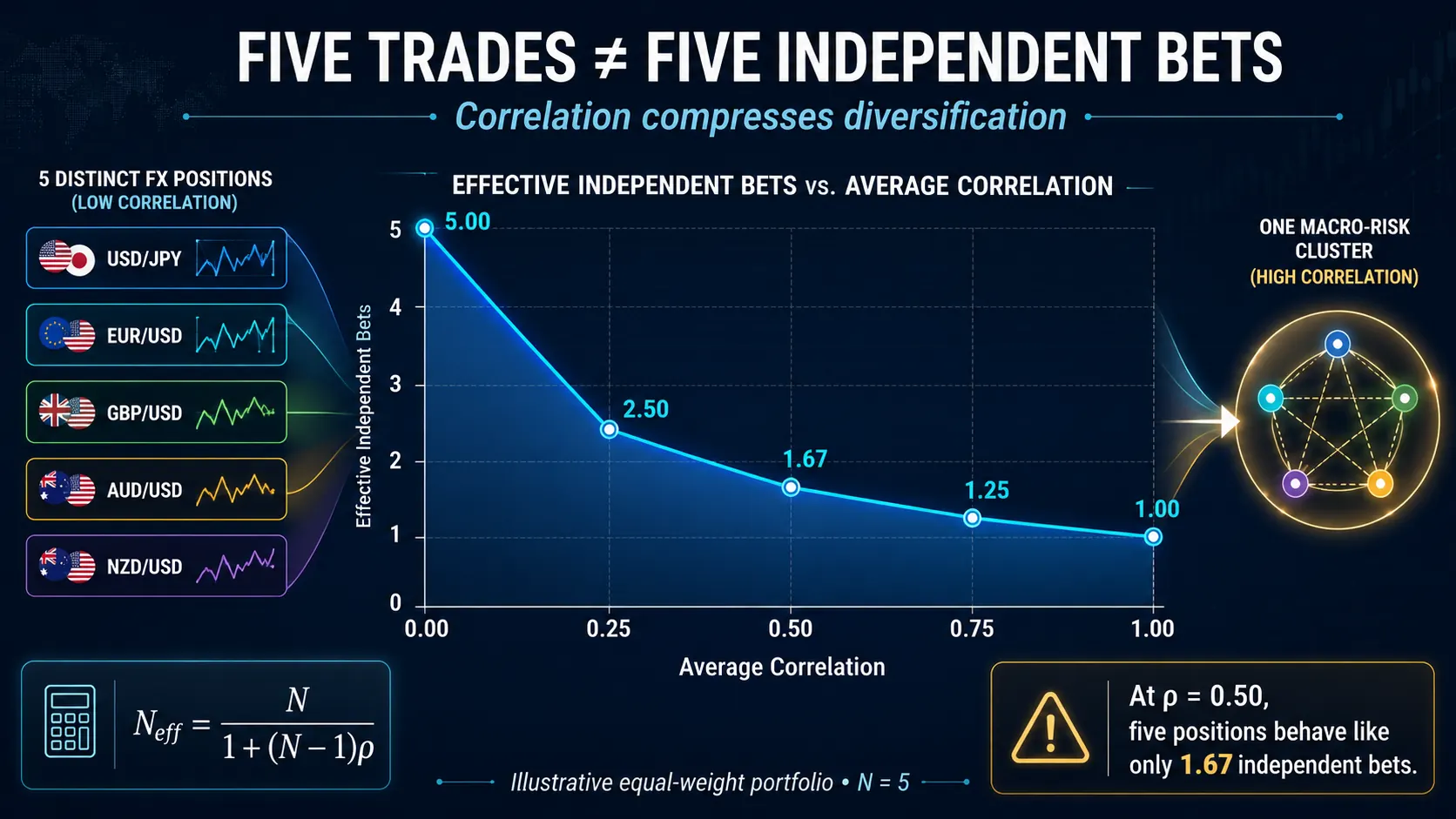
This metric is deliberately humbling. It prevents a trader from claiming diversification merely because a terminal displays several symbols. It also highlights a subtle point: concentration is not automatically bad. If the trader intentionally wants one strong USD thesis, then 1.43 effective bets may be acceptable—but the position cluster should be sized and governed as one thesis, not four unrelated opportunities.
Use Concentration Measures That Answer Different Questions
No single metric captures every form of portfolio concentration. A practical dashboard combines several measures, each with a specific job.
Gross portfolio heat
Gross heat is the sum of initial risk across open positions. It answers: how much equity is at risk if every stop is hit? It is simple and conservative, but it ignores offsets and correlation. That limitation is acceptable because gross heat is a capacity control, not a complete model.
Net currency exposure
Net exposure sums the long and short legs by currency. It answers: which currency direction dominates? Netting must be interpreted carefully. A long EUR/USD and short EUR/JPY offset some EUR direction, but they do not necessarily offset event risk, volatility risk, or execution timing. Mathematical netting can hide basis differences between the two pairs.
Herfindahl-Hirschman concentration index
The HHI is the sum of squared portfolio shares: HHI = Σpᵢ². If four independent clusters each hold 25% of the portfolio risk, HHI is 0.25 and 1/HHI equals four effective equally weighted clusters. If one cluster holds 70% and three hold 10% each, HHI rises to 0.52 and the inverse falls to 1.92. HHI measures allocation concentration, but it does not know that two nominally different clusters may still be correlated.
Marginal risk contribution
Marginal contribution asks how much total portfolio risk changes when a position is added, removed, or resized. This is superior to pair-by-pair thinking because a 0.50% trade can contribute very little if it offsets an existing exposure—or a great deal if it reinforces the portfolio's dominant factor. The decision is not “Is this setup good?” but “What does this setup do to the whole book?”
| Measure | Best question | Blind spot | Use in practice |
|---|---|---|---|
| Gross heat | Worst case if stops are reached? | Ignores diversification | Hard account capacity limit |
| Currency vector | Which currency direction dominates? | Ignores nonlinear co-movement | Per-currency directional caps |
| Correlation risk | How much may positions move together? | Estimate changes by regime | Cluster sizing and stress tests |
| HHI / inverse HHI | How concentrated are risk shares? | Does not model correlation | Allocation balance check |
| Marginal contribution | What does the next trade add? | Needs stable covariance inputs | Accept, reduce, replace, or reject |
A Worked Example: Good Setups, Bad Portfolio
Assume an intraday trader identifies four technically valid setups during the London session. Each risks 0.50% of equity. Individually, every chart meets the entry plan. The portfolio decision is still poor if the trader ignores shared exposure.
| Trade | Setup | Currency driver | Regime need | Added portfolio effect |
|---|---|---|---|---|
| Long EUR/USD | Breakout-retest | Short USD | Trend expansion | Creates initial USD cluster |
| Long GBP/USD | Momentum continuation | Short USD | Trend expansion | Reinforces same direction |
| Long AUD/USD | Range break | Short USD + risk-on | Expansion | Adds USD and sentiment overlap |
| Short USD/JPY | Yield-led breakdown | Short USD | Lower U.S. yields | Completes four-trade USD thesis |
The naive view says the account has four 0.50% trades and therefore 2.00% gross risk. The portfolio view adds three more facts: all four are short USD, all were opened in the same session, and all need directional continuation. If a U.S. data surprise strengthens the dollar while volatility expands, the positions can move against the trader together and experience slippage together.
A better response is not necessarily to reject every trade. The trader could choose the cleanest one, split a single cluster budget among two or three expressions, replace one position with a genuinely different driver, or wait until the first position is protected before adding another. The key is that the cluster receives one risk budget.
Resize the cluster, not just the tickets
Suppose the trader's approved risk for one directional cluster is 1.00% of equity. Four signals do not create four separate 1.00% permissions. They compete for the same cluster budget. The simplest allocation is 0.25% per trade, but equal sizing is not mandatory. The cleanest pair might receive 0.40%, two secondary expressions 0.25% each, and an event-sensitive position only 0.10%. Gross ticket risk still sums to the authorized 1.00%.
A more refined allocation uses marginal contribution. Start with the strongest trade, then add each candidate to the covariance or stress model. If the second trade adds substantial expected value but only modest incremental risk, it deserves capacity. If the third trade contributes nearly the same downside as the first while adding little independent payoff, its size should be cut or its place given to another exposure. This forces the portfolio to earn the right to become more complex.
Sequencing is another control. A trader may open the first position at planned risk, then permit a second only after the first reaches a defined protection state—such as a reduced stop, partial exit, or invalidation of the shared catalyst. Sequencing does not make correlation disappear, and moving a stop to breakeven does not eliminate gap or slippage risk, but it can prevent all cluster members from carrying maximum fresh risk simultaneously.
Concentration changes the loss distribution
The danger of concentration is not merely a larger average losing day. It changes the shape of the return distribution. Correlated positions produce more loss clustering, fatter left-tail outcomes, faster drawdown velocity, and a heavier recovery burden. Four isolated 0.50R losses spread across a month can be absorbed psychologically and financially very differently from four 0.50R losses triggered within minutes by one event.
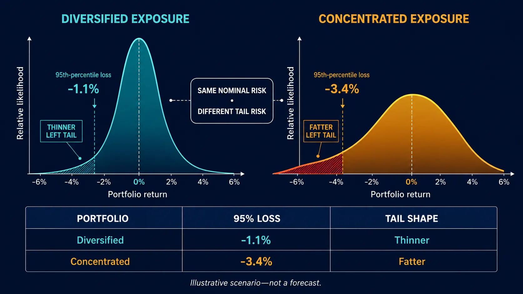
It can also distort performance attribution. A trader may count four losing trades and conclude that four setup types failed. In reality, one portfolio-level thesis failed and was expressed four times. If the journal grades each ticket independently, the trader may overestimate the sample size, underestimate common-factor exposure, and make the wrong strategy changes. Portfolio episodes should therefore be tagged alongside individual trades so one macro event is not mistaken for four independent pieces of evidence.
When Concentration Is Rational
Diversification is not a moral virtue, and concentration is not automatically reckless. A portfolio can become so diluted that the best idea is barely expressed, costs multiply, and low-quality trades are added only to create the appearance of balance. Intentional concentration can be rational when evidence, liquidity, and governance support it.
The standard should be higher, however. A concentrated cluster should have a clearly stated thesis, a defined invalidation mechanism, a known catalyst calendar, a total cluster-risk limit, and a plan for correlation stress. It should also offer something beyond duplicate exposure. Two positions may express the same macro view but differ in relative strength, payoff asymmetry, execution quality, or liquidity. If the second trade adds no meaningful improvement, it is probably duplication rather than diversification.
Strong opinion. If you cannot explain why the second correlated trade improves the portfolio, it probably does not belong in the portfolio.
Build a Portfolio Concentration Policy
A usable concentration policy should be short enough to apply before execution and specific enough to stop rationalization. The limits below are examples, not recommendations. They must be calibrated to account size, leverage, strategy expectancy, holding period, broker conditions, and drawdown tolerance.
| Control | Illustrative rule structure | Decision if limit is approached |
|---|---|---|
| Account heat | Maximum total initial risk across all open trades | Reduce size or wait for risk to come off |
| Currency cap | Maximum long or short exposure to one currency | Choose the best expression; reject duplicates |
| Cluster cap | Maximum risk to one macro or strategy thesis | Split a single budget across cluster members |
| Event cap | Lower allowed risk near tier-one releases | Cut, hedge, or pause additions |
| Session cap | Limit new correlated exposure in one session | Stagger entries or require protection first |
| Stress multiplier | Recalculate with higher assumed correlation/slippage | Use stressed risk for approval |
| Drawdown throttle | Tighten every cap as account state weakens | Concentration authority contracts with capital authority |
A five-step pre-trade workflow
- 1. Decompose. Translate the proposed pair into long and short currency legs.
- 2. Aggregate. Update gross heat, net currency exposure, and cluster totals.
- 3. Stress. Assume correlation rises, spreads widen, and the common catalyst moves against the book.
- 4. Compare. Measure marginal risk contribution against the trade's expected benefit.
- 5. Decide. Accept, resize, replace, sequence, hedge, or reject the trade.
Design the Dashboard Around Budget Utilization
A concentration dashboard should not merely display red and green correlations. It should show how much of each risk budget is already consumed. The most useful columns are current exposure, approved limit, utilization percentage, stress utilization, and the marginal effect of the next proposed trade.
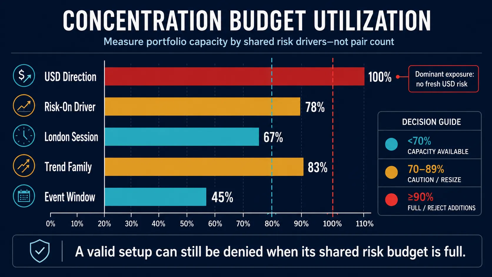
This presentation converts analysis into action. A 0.72 correlation is intellectually interesting; “adding this trade moves USD-direction utilization from 82% to 108%” is operationally decisive. The dashboard should also distinguish current risk from fresh-risk capacity. A protected or partially closed trade may free some capacity, but only if the remaining position's gap, slippage, and event risks are still represented honestly.
Common Concentration Mistakes
Mistake 1: Using pair count as a diversification score
Ten pairs can contain one dollar factor, one carry factor, or one global risk-sentiment factor. Count the underlying exposures and failure mechanisms instead.
Mistake 2: Treating historical correlation as a law
Correlation is sample-dependent and regime-dependent. Use rolling estimates, stress assumptions, and structural overlays. A low recent correlation does not cancel an obvious shared catalyst.
Mistake 3: Netting away risk too aggressively
Opposite currency legs can reduce directional exposure without eliminating spread risk, timing risk, basis risk, or strategy risk. A partial offset is not the same as a closed position.
Mistake 4: Ignoring strategy concentration
A portfolio of different currencies can still be concentrated in one fragile behavior: every trade may depend on breakouts following through, volatility remaining elevated, or mean reversion returning quickly. Strategy-family correlation often appears only when the regime changes.
Mistake 5: Adding risk because earlier trades are profitable
Open profit does not automatically create new risk authority. If all positions share one driver, adding after a favorable move can increase late-stage trend and reversal risk. Recalculate the portfolio after stop movement, partial exits, and new entries rather than relying on the feeling that the account is playing with house money.
Mistake 6: Setting universal limits without evidence
A one-size concentration cap can be too loose for a high-variance system and too restrictive for a low-risk, market-neutral structure. Limits should be tested against historical portfolios, slippage, loss clustering, Monte Carlo paths, and the trader's actual execution behavior.
Review Concentration at Three Speeds
Portfolio concentration changes faster than most risk manuals acknowledge. The right review cadence has three levels.
| Cadence | Primary job | What to update |
|---|---|---|
| Pre-trade / live | Prevent accidental clustering | Currency vector, heat, cluster utilization, event risk, marginal contribution |
| Daily / weekly | Diagnose realized joint behavior | Loss clusters, rolling correlation, concurrent MAE, slippage, strategy overlap |
| Monthly / quarterly | Calibrate the architecture | Caps, stress assumptions, regime shifts, factor definitions, diversification benefit |
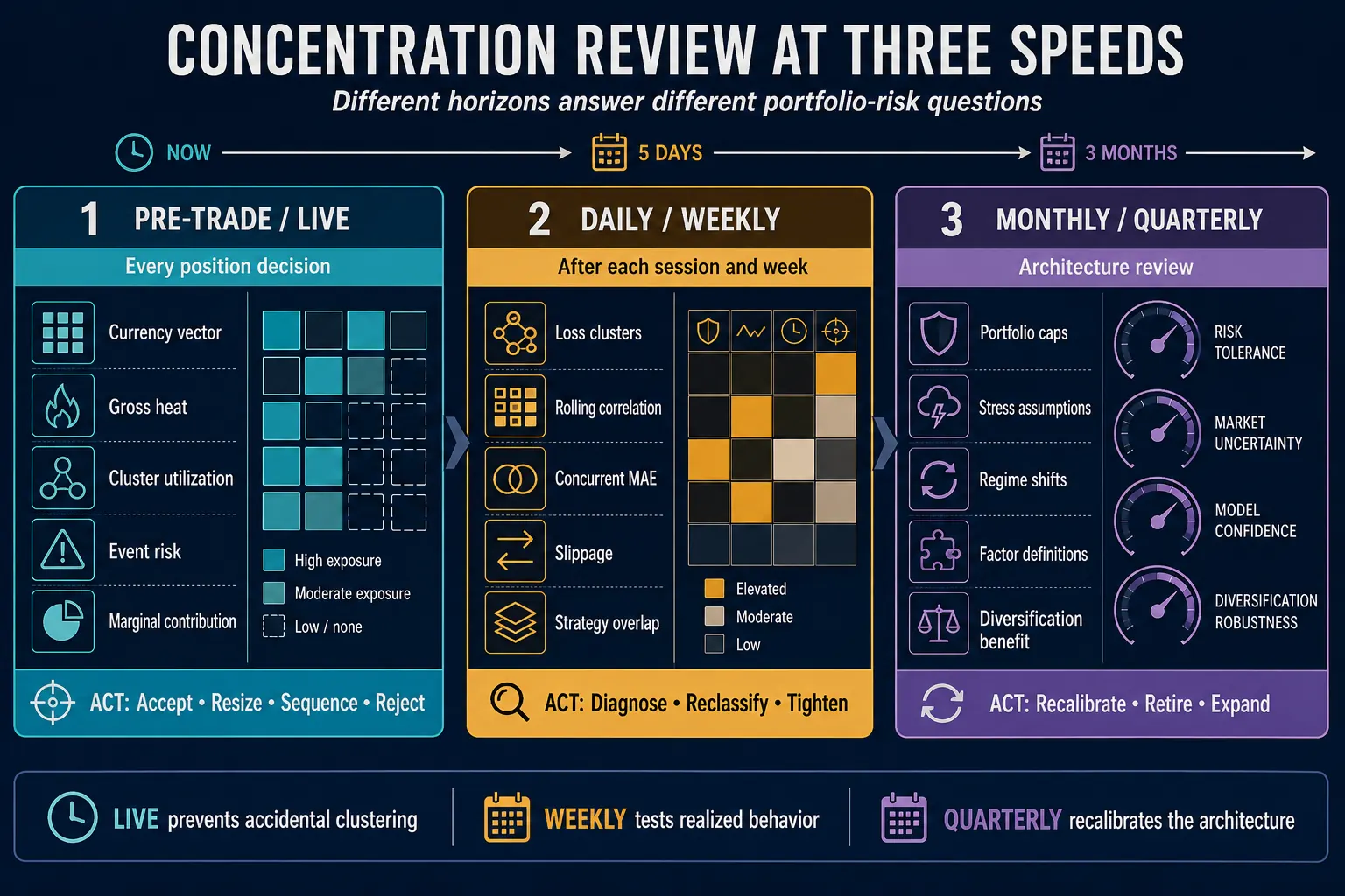
The weekly review is especially valuable. Compare expected diversification with realized diversification. Did supposedly independent trades reach maximum adverse excursion at the same time? Did spread expansion or news slippage hit several positions together? Did one currency, session, or strategy family produce most of the drawdown? These observations should feed back into cluster definitions and stress multipliers.
At the longer horizon, evaluate whether diversification actually improved risk-adjusted results. More symbols can increase trading costs and operational complexity without improving expectancy. The objective is not maximum variety. It is the smallest set of exposures that delivers robust, nonredundant sources of return within a survivable risk budget.
The Portfolio Manager's Final Test
Before approving a new FX position, ask one final question: If this trade loses, what else is likely to be losing at the same time? That question forces the trader to leave the chart and inspect the book.
Portfolio concentration is ultimately an authority problem. A setup can be valid while the portfolio is already full. A high-conviction macro thesis can be correct while its risk expression is duplicated. A new trade can have positive standalone expectancy while reducing portfolio quality because it adds more downside than independent edge.
Professional portfolio management begins when the account stops treating every signal as an isolated opportunity. The unit of decision becomes the total exposure: currencies, drivers, strategies, timing, volatility, and operational dependencies. Once those layers are measured together, concentration becomes intentional, budgeted, and reviewable instead of accidental.
Bottom line. The goal is not to eliminate concentration. The goal is to know exactly where it is, why it is there, how much capital authority it has, and what must happen for it to be reduced.
Key Takeaways
| # | Principle |
|---|---|
| 1 | Pair count is not diversification; shared failure paths determine concentration. |
| 2 | Decompose every pair into currency legs and aggregate a portfolio exposure vector. |
| 3 | Combine gross heat, currency exposure, correlation, HHI, and marginal contribution. |
| 4 | Treat correlated positions as a cluster with one risk budget. |
| 5 | Stress correlation, slippage, and common catalysts before adding a trade. |
| 6 | Review concentration live, weekly, and at the architecture-calibration horizon. |
Sources and Further Reading
- U.S. Commodity Futures Trading Commission. Eight Things You Should Know Before Trading Forex
- Bank for International Settlements. OTC Foreign Exchange Turnover in April 2025
- Basel Committee on Banking Supervision. MAR21: Standardised Approach — Sensitivities-Based Method
- Bank for International Settlements. Hedge Fund Exposure to the Carry Trade
- CME Group. CME SPAN 2 Margin Framework
Educational note. This article explains portfolio-risk concepts for educational purposes. Illustrative figures and thresholds are not investment advice or personalized risk recommendations.