

Core thesis. An equity curve is not a single object. It is a return path observed through a chosen clock and denominator. Change either one and the apparent quality of the strategy can change without changing a single trade.
The Same Curve Can Tell Three Different Stories
Most strategy reviews begin with a cumulative line plotted against trade number. The visual is clean: left to right, up or down, with drawdowns cut into the slope. For an advanced forex evaluator, however, that picture is only the sequencing view. It says how outcomes accumulated in the order trades closed. It does not say how long capital waited, how much risk was occupied between closes, how external cash flows distorted the account balance, or how much of the gross edge leaked through spread, commission, slippage, financing, and rollover.
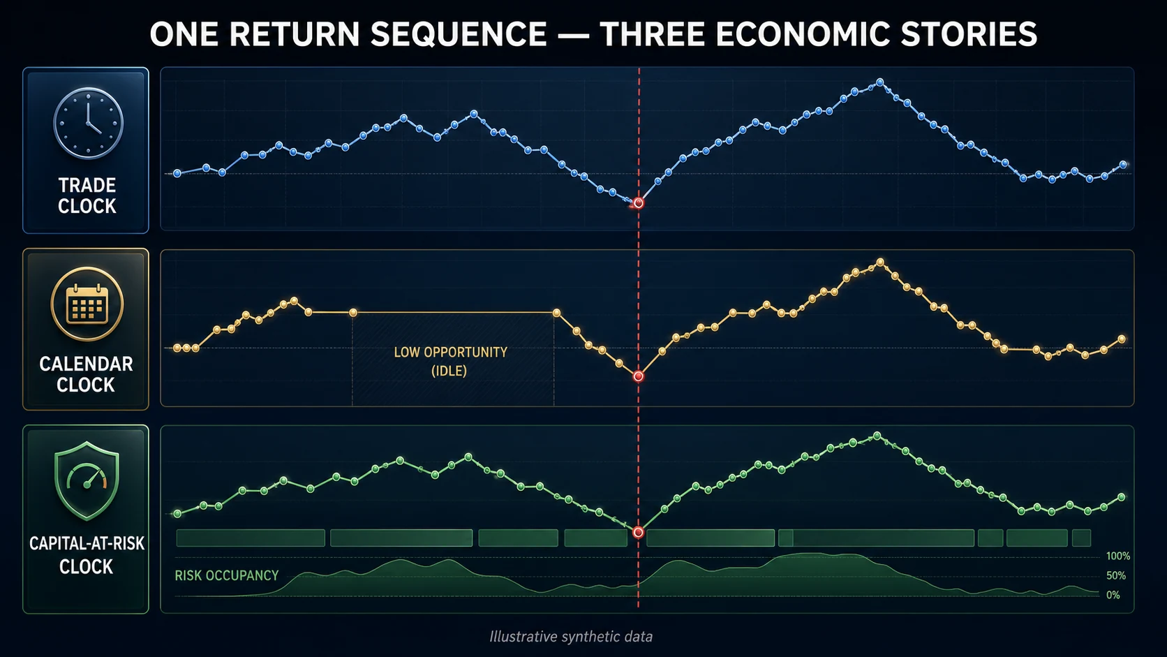
That distinction matters in foreign exchange because strategies can express identical statistical expectancy through radically different operating geometries. A London-session scalper may realize hundreds of short-duration bets, a multi-day carry process may hold a handful of positions across rollover, and a macro swing model may remain flat for weeks before committing concentrated risk. Plot all three against trade number and the inactive calendar disappears. Plot all three against calendar time and differences in opportunity frequency dominate. Plot them against capital-at-risk time and a third ranking can emerge.
The practical implication is uncomfortable: a visually superior trade-index curve can be an inferior business. It may require more calendar time, more continuous margin occupancy, greater weekend gap exposure, or a cost structure that compounds against the edge. Conversely, a lumpy curve may be economically efficient if it earns its return with limited risk occupancy and survives realistic execution.
The framework below treats equity-curve analysis as a controlled reconstruction problem. First clean the path. Then choose the denominator. Then choose the clock. Only after those decisions should the evaluator interpret slope, drawdown, smoothness, and persistence.
Why the Trade-Order Curve Is So Seductive
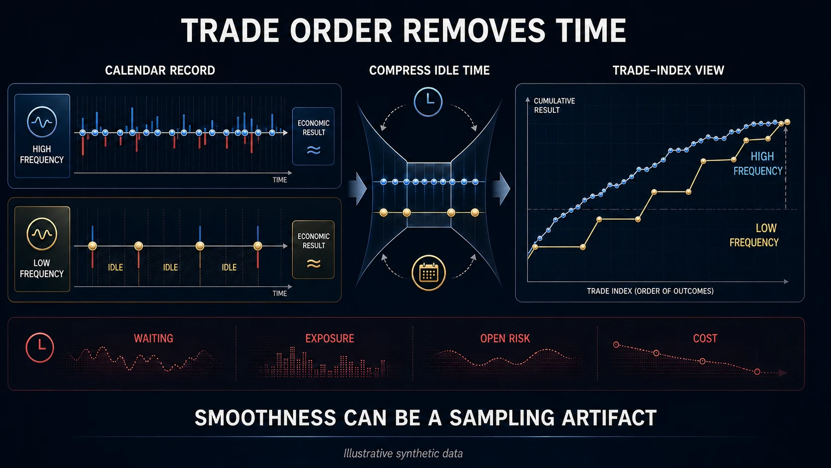
Trade order removes idle time and makes strategies with different frequencies look directly comparable. That is useful when the question is narrow: does the sequence exhibit positive drift, loss clustering, outlier dependence, or a change in payoff behavior? The problem begins when the evaluator lets the same curve answer questions it was never built to answer.
A trade-index slope is return per completed observation. It is not return per month, return per unit of risk capital, or return per hour exposed. A smooth curve can therefore be manufactured by frequency. If a process makes many small bets, the x-axis stretches every small outcome into its own step; if another process makes fewer large bets, each outcome occupies more visual space. Smoothness can be a sampling artifact rather than evidence of superior edge quality.
The same problem appears in drawdown duration. A 40-trade recovery can mean two weeks for one model and fourteen months for another. Expressed only in trades, the first looks no different from the second. Expressed only in days, a low-frequency process may look stagnant even when it is behaving exactly as designed. The solution is not to choose the one correct axis. It is to require several axes to agree.
The Three Clocks
1. Trade clock: what happened per decision
The trade clock indexes realized outcomes by completed trade or decision unit. It is the best view for payoff sequencing, streak structure, tail contribution, and whether the edge is concentrated in a small number of observations. Use it to inspect cumulative R, rolling expectancy, hit-rate stability, average win and loss, and the contribution of the largest winners. If five trades create the entire curve, the curve is not yet evidence of a broadly distributed process; it is evidence that five outcomes mattered.
For portfolios, the decision unit requires discipline. One ticket is not always one independent bet. EUR/USD long, GBP/USD long, and USD/CHF short may close at different times but share a dominant short-dollar exposure. Counting them as three unrelated observations can inflate the apparent information in the curve. Grouping economically linked entries into campaign or risk-event units often produces a more honest trade clock.
2. Calendar clock: what happened to the business over time
The calendar clock preserves opportunity gaps, market closures, slow regimes, and the waiting burden imposed on capital and the operator. It answers whether the strategy is deployable at the required return horizon. A fund, proprietary account, or self-funded trader experiences rent, financing, benchmark pressure, and attention costs in calendar time, not in trade count.
Calendar curves should be marked to market at a consistent frequency. Closed-trade balance is inadequate whenever open P&L is material. A strategy can show a clean realized balance while carrying a deep floating drawdown; the apparent stability exists only because losses have not yet been crystallized. Daily end-of-day equity is usually the minimum serious surface for multi-day FX strategies, with higher-frequency marks justified when intraday margin calls or stop-out risk matter.
3. Capital-at-risk clock: what happened while risk was actually occupied
The risk clock accumulates exposure rather than wall time. A simple version is exposure-days: sum the fraction of authorized risk capital that was active during each day. A position carrying 0.75% initial risk for two days contributes 1.5 risk-percent-days; two concurrent positions at 0.50% each contribute 1.0 risk-percent-day for every day both remain open. More sophisticated implementations can use expected shortfall, volatility target, margin utilization, or portfolio risk contribution as the occupancy measure.
This view is not a replacement for calendar returns. It is a capacity lens. It asks how efficiently a strategy converts occupied risk into outcome. A low-frequency process that earns 12R while barely using its risk budget may be highly efficient but under-deployed. A high-frequency process that earns 15R while continuously consuming the full budget may be less attractive once capacity, operational load, and correlation with other strategies are considered.
Each clock is valid, but only for the question encoded in its denominator.
| Clock | Denominator | Best question | Primary failure mode exposed |
|---|---|---|---|
| Trade | Completed decision units | Is the payoff sequence broad, stable, and repeatable? | Outlier dependence; streaks; weak effective sample |
| Calendar | Days / weeks / months | Is the return path deployable at the required horizon? | Stagnation; long recovery; hidden open-equity stress |
| Risk | Exposure-days or risk-budget time | How efficiently does occupied risk produce return? | Capital congestion; concurrency; low capacity efficiency |
Normalize the Path Before Interpreting It
Neutralize cash flows
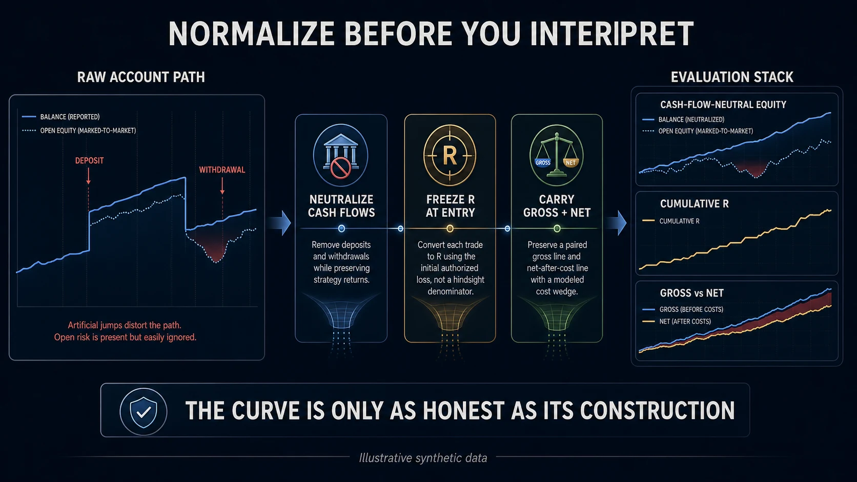
Deposits and withdrawals can create false acceleration, false recovery, and false drawdown. For strategy comparison, build a cash-flow-neutral return series. Time-weighted return methods segment the record around external cash flows so the manager or strategy is not credited for contributed capital. The GIPS standards formalize this logic for performance presentation, including valuation around large external cash flows. A retail FX account does not become exempt from the arithmetic because the cash flow came from the owner.
Maintain both views: actual account equity for solvency and operational control, and cash-flow-neutral indexed equity for evaluation. The first answers whether the account can survive; the second answers what the strategy did.
Choose a stable risk denominator
Account-percent curves mix edge with sizing policy. If risk per trade changes, the curve changes even if the underlying trade outcomes in R are identical. That is valuable when assessing the complete production system, but destructive when comparing signal or management quality. Build a cumulative R curve using the initial authorized loss for each decision unit, then separately reconstruct the account curve under the actual sizing policy.
The denominator must be frozen at decision time. Recalculating R from the final stop after discretionary widening, or from account equity after the outcome is known, retrofits the unit to the result. The point of R-normalization is to preserve what the process authorized before uncertainty resolved.
Carry gross and net curves together
In FX, the net curve is not simply the gross curve shifted downward by a fixed annual fee. The wedge depends on turnover, spread state, order type, time of day, volatility, liquidity, trade size, and holding period. BIS research describes FX execution as highly fragmented and shows how spreads and execution methods reflect liquidity and market-risk transfer. That makes transaction drag conditional, not constant.
At minimum, reconstruct four layers: theoretical signal price; executable bid/ask price; realized fill including slippage and rejection effects; and financed outcome including commission and swap. If the gross edge survives while the realized edge decays, the equity curve is diagnosing execution infrastructure rather than strategy logic.
Drawdown Is an Event, Not a Number
Maximum drawdown compresses a path into one peak-to-trough coordinate. It is necessary, but radically incomplete. Two strategies can share the same 12% maximum drawdown while differing in decline speed, time spent underwater, recovery time, number of failed recovery attempts, and the concentration of losses by currency, session, or regime. Formal drawdown research likewise treats the underwater process as a path-dependent object rather than ordinary symmetric volatility.
Represent every drawdown as an event record with at least seven fields: prior peak date; trough date; recovery date; depth; time to trough; time from trough to recovery; and cumulative risk occupancy during the event. Then add attribution: which pairs, strategy branches, regimes, cost states, and discretionary overrides contributed. A drawdown lasting 90 days with only eight days of active risk tells a different story from one lasting 90 days under continuous exposure.
Time under water should also be measured as a proportion of the full sample. A strategy that is below its prior high for 75% of the record can still be profitable, but it imposes a different governance and behavioral burden from one that resets highs frequently. That burden belongs in the evaluation because capital may be withdrawn, risk may be throttled, or the strategy may be abandoned before long-run expectancy appears.
Read Slope as a Conditional Rate
Equity slope is often described as if it were an intrinsic property of a strategy. It is actually a rate: return divided by the chosen horizontal unit. The evaluator should therefore report several rates side by side: R per 100 trades; cash-flow-neutral return per year; R per exposure-day; return per unit of average portfolio risk; and net return after costs. No single rate deserves to dominate every allocation decision.
Then condition those rates. In FX, aggregate slope can be carried by one volatility state, one currency family, one session, or one monetary-policy regime. Create contribution curves by regime and subtract them from the total. If removing a single state eliminates most of the long-run drift, the strategy may be a regime specialist rather than a general edge. That is not automatically a defect, but it changes the mandate, allocation, and suspension rules.
Avoid mechanically ranking slopes with a naïvely annualized Sharpe ratio. Andrew Lo showed that serial correlation can materially distort Sharpe annualization and even strategy rankings. The problem is especially relevant when returns are smoothed by stale marks, overlapping positions, multi-day holding periods, or closed-trade accounting. A strategy that reports weekly returns from positions held for several weeks does not produce independent weekly observations merely because the spreadsheet has one row per week.
A Worked Comparison: When the Ranking Reverses
Consider three hypothetical FX strategies evaluated over the same two-year window. The numbers below are intentionally illustrative; their purpose is to show how rankings change when the denominator changes.
| Metric | A: Session scalper | B: Swing trend | C: Event mean reversion | Naïve winner | What the metric misses |
|---|---|---|---|---|---|
| Cumulative trade-index R | 42R | 31R | 27R | A | Time, capacity, and cost |
| Net cash-flow-neutral return | 18% | 24% | 15% | B | Different risk budgets |
| R per 100 trades | 7.0 | 17.2 | 15.0 | B | Opportunity frequency |
| R per 100 exposure-days | 5.1 | 8.4 | 13.7 | C | Idle capital may be useful elsewhere |
| Maximum drawdown | −9.8% | −12.1% | −8.9% | C | Duration and recovery burden |
| Median recovery time | 18 days | 96 days | 41 days | A | Tail recovery event |
| Gross-to-net retention | 61% | 88% | 82% | B | Execution model uncertainty |
| Largest regime contribution | 44% | 63% | 38% | C | Regime classification error |
A dominates the raw trade-index curve but surrenders much of the edge to turnover-dependent costs. B is strongest in annual net return and per-trade productivity but carries a long recovery burden and concentrated regime dependence. C produces the least total R yet converts occupied risk efficiently and diversifies the other two. A serious allocation decision might fund all three at different weights — or reject A if its execution assumptions cannot be validated. The point is that the original equity ranking is not the conclusion. It is the first observation.
Put Uncertainty Around the Curve
A single realized path is one draw from a distribution of possible paths. Smoothness can be sequence luck. A strategy with positive expectancy can experience a poor realized order; a weak strategy can receive a flattering order. Bootstrap or Monte Carlo analysis should preserve the dependence structure that matters — trade clustering, serial correlation, regime blocks, and overlapping exposure — rather than shuffling every trade as if outcomes were independent.
Plot percentile bands for terminal outcome, maximum drawdown, drawdown duration, and time under water. Then place the live curve inside the same coordinate system used for the simulation. If live results drift toward an adverse percentile, do not automatically declare edge decay; first test whether execution cost, exposure mix, or regime occupancy changed. The curve should trigger attribution, not diagnosis by itself.
Selection history also belongs around the curve. If the displayed strategy was chosen from hundreds of variants, the best-looking path inherits selection bias. The Deflated Sharpe Ratio was developed to adjust for non-normal returns and multiple testing, while the Probability of Backtest Overfitting framework evaluates how often selection procedures choose configurations that disappoint out of sample. An evaluator should record the number of trials, parameter families, rejected variants, and selection rule — not merely the champion curve.
Forex-Specific Failure Modes
- Closed-trade equity hiding floating loss. Reconstruct marked-to-market equity at a frequency consistent with the risk horizon.
- Pair count masquerading as diversification. Aggregate exposure by currency and macro driver before interpreting smoothness.
- Rollover and financing omitted from longer-horizon paths. Attribute swap separately so carry is not confused with directional alpha.
- Spread modeled as a constant. Use time-of-day, volatility, size, and event-conditioned cost assumptions where data permit.
- Timezone boundaries creating artificial daily returns. Fix the valuation cut and test sensitivity around rollover and session transitions.
- Deposits creating false new highs. Maintain operational account equity and cash-flow-neutral evaluation equity as separate series.
- Overlapping positions inflating sample size. Use campaign, cluster, or risk-event units and adjust inference for dependence.
- Regime labels defined after seeing the curve. Freeze classification rules before using them for performance attribution.
The Equity-Evidence Stack
The complete review can be organized as four layers. Failure at an early layer invalidates interpretation at every later layer. A beautiful chart cannot rescue contaminated cash flows; sophisticated attribution cannot rescue a denominator that changes after outcomes are known.
- 1. Clean the path. Remove deposits and withdrawals; mark open risk to market; preserve timestamps.
- 2. Choose the denominator. Account percent, R-multiples, volatility budget, and risk capital answer different questions.
- 3. Choose the clock. Trade count, calendar time, and capital-at-risk time reveal different constraints.
- 4. Attribute and challenge. Costs, regimes, concentration, uncertainty bands, and out-of-sample evidence.
Only after all four layers agree should the curve influence capital authority.
A Governance Decision Ladder
Equity analysis becomes useful only when observations map to controlled decisions. The following ladder keeps the cumulative line from becoming an emotional permission slip.
- 1. Observe. Update trade-, calendar-, and risk-clock panels. Confirm data completeness and valuation consistency.
- 2. Reconcile. Explain differences between balance, marked-to-market equity, cash-flow-neutral equity, gross curve, and net curve.
- 3. Attribute. Partition the change by pair, currency exposure, regime, session, strategy branch, costs, and discretionary overrides.
- 4. Challenge. Compare the path with out-of-sample expectations and dependence-aware simulation bands. Account for the research-selection history.
- 5. Authorize. Maintain, throttle, suspend, or increase capital only under predefined evidence thresholds. Separate research changes from production controls.
Decision rule. Never allocate because the curve looks smooth. Allocate because the clean, net, marked-to-market path remains credible across the clocks and denominators relevant to the mandate.
Final Perspective: The Curve Is a View, Not the Strategy
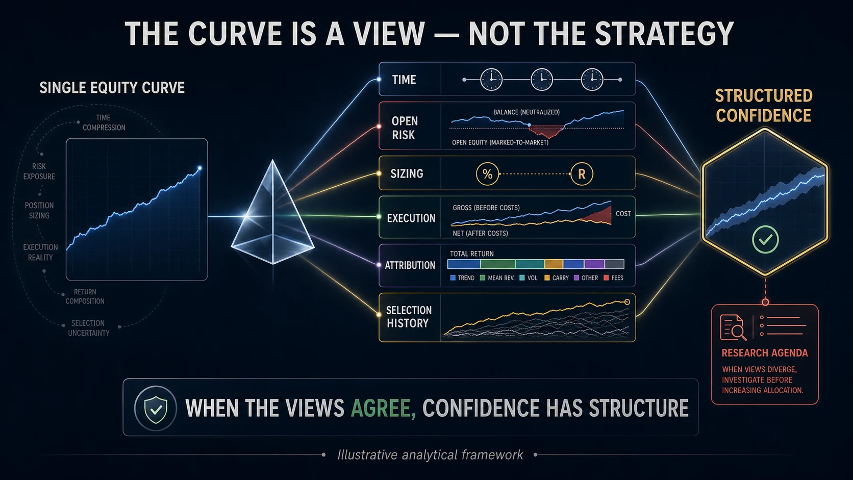
Advanced equity-curve analysis is not the art of finding more indicators to place under a line. It is the discipline of asking what was removed when the line was constructed. Trade-order curves remove time. Balance curves may remove open risk. Dollar curves mix edge with sizing. Gross curves remove execution. Aggregate curves remove attribution. Backtest champions remove the losing research history.
A defensible strategy evaluation restores those missing dimensions. It rebuilds the path after cash flows, marks open positions, carries gross and net outcomes together, freezes the risk denominator, and reads the result through trade, calendar, and capital-at-risk clocks. It treats drawdown as an event with depth, duration, recovery, and exposure geometry. It challenges smoothness with uncertainty bands and selection-aware statistics.
The result is not one prettier equity curve. It is a set of mutually constraining views. When they agree, confidence has structure. When they disagree, the disagreement is the research agenda.
Methodology Note
All numerical examples and charts in this article are original, deterministic synthetic illustrations created for explanation. They do not represent Montex AlphaRail customer results, a tradable strategy, broker data, or expected performance. Metrics are shown to demonstrate how rankings and diagnoses change under different clocks, denominators, and cost assumptions.
Sources and Further Reading
The article draws on the following research and industry sources. Accessed August 31, 2026.
- CFA Institute. Global Investment Performance Standards (GIPS) — input data and calculation methodology
- Schrimpf, Andreas; Sushko, Vladyslav. FX Trade Execution: Complex and Highly Fragmented — BIS Quarterly Review, December 2019
- BIS Markets Committee. FX Execution Algorithms and Market Functioning — Markets Committee Papers No. 13
- Chekhlov, Alexei; Uryasev, Stanislav; Zabarankin, Michael. Drawdown Measure in Portfolio Optimization
- Lo, Andrew W. The Statistics of Sharpe Ratios
- Bailey, David H.; López de Prado, Marcos. The Deflated Sharpe Ratio: Correcting for Selection Bias, Backtest Overfitting and Non-Normality
- Bailey, David H.; Borwein, Jonathan M.; López de Prado, Marcos; Zhu, Qiji Jim. The Probability of Backtest Overfitting
- Bank for International Settlements. Triennial Central Bank Survey of Foreign Exchange and OTC Derivatives Markets in 2022
- Montex AlphaRail. Blog & Insights archive — reviewed August 31, 2026 for editorial differentiation
Risk disclosure. Trading foreign exchange and leveraged instruments carries substantial risk and may not be suitable for all investors. This article is educational and analytical; it does not provide investment advice, trading signals, or any guarantee of profitability. Past, hypothetical, and simulated performance are not reliable indicators of future results.