

Your trading platform counts tickets. A risk engine counts economic bets.
Four positions can have four symbols, four entry signals, and four stop-loss orders — and still depend on the same currency move. When that shared factor reverses, apparent diversification disappears precisely when the portfolio needs it most.
The Portfolio Illusion
A trader opens long EUR/USD, long GBP/USD, short USD/JPY, and long XAU/USD. On the screen, the positions look different. They involve Europe, Britain, Japan, and gold. They may even come from different technical setups. But economically, all four positions lean in the same direction: they benefit from a weaker U.S. dollar.
That is the correlation-risk problem in its most practical form. The portfolio contains four execution events but may contain only one dominant macro thesis. If dollar strength arrives — perhaps after a rate surprise, a flight to liquidity, or a broad repricing of U.S. yields — the positions can deteriorate together. The trader did not build four independent opportunities. The trader multiplied one exposure across four instruments.
This distinction matters because portfolio risk is not the sum of position labels. It is the interaction among direction, size, volatility, currency legs, holding period, exit logic, and the market regime. A professional risk process therefore asks a different question before every new trade: What new risk factor does this position add to what is already open?
Trade Count Is Not Diversification
Diversification exists only when positions respond differently enough to the forces that drive their profit and loss. Owning several symbols is cosmetic diversification if those symbols share the same underlying driver. In foreign exchange, this happens constantly because every currency pair contains two legs and the same major currencies recur across the portfolio.
A long EUR/USD position is simultaneously long euros and short U.S. dollars. A long GBP/USD position is long pounds and short dollars. A short USD/JPY position is short dollars and long yen. The symbols differ, but the dollar leg points the same way in all three. Add long gold priced in dollars, and the portfolio may acquire a fourth expression of the same dollar-weakness theme.
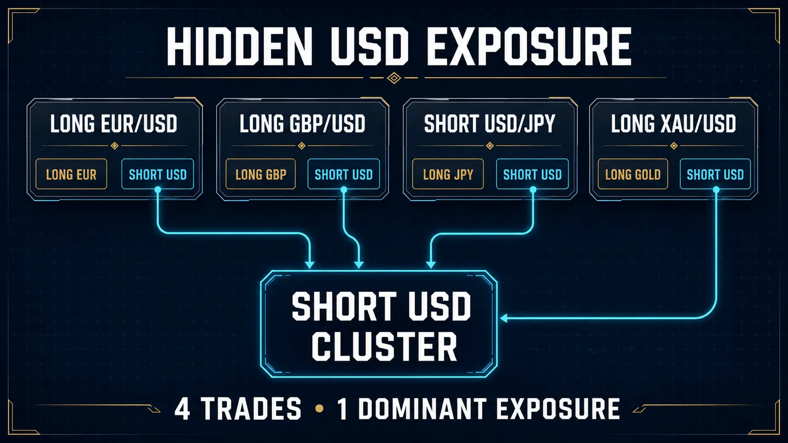
The dangerous assumption is: four 1% trades equal four separate 1% risks. The correct interpretation is more conditional. The hard planned loss is still 4% if every trade reaches its stop and fills as intended. Correlation does not change that arithmetic ceiling. What correlation changes is the probability that losses occur together, the speed at which drawdown accumulates, and the chance that several stops are stressed by the same event.
Nominal open risk measures how much could be lost if stops are reached under the sizing assumptions. Correlation risk measures how likely positions are to win, lose, or become volatile together. It changes clustering and portfolio behavior — not the basic addition of the stop-loss budgets.
The Four Layers of Correlation Risk
A single correlation coefficient is too blunt for serious portfolio control. Intermediate and advanced traders should separate at least four related but distinct layers.
1. Instrument-return correlation
This is the familiar relationship between two instruments over a selected window. It is useful but sensitive to timeframe, sample length, session, and regime; a calm daily estimate can conceal strong intraday co-movement.
2. Signed trade-P&L correlation
This is closer to what the portfolio experiences because direction is included. Raw pair prices can be negatively correlated while the selected long and short positions still produce positively related P&L. A risk engine should correlate signed returns or strategy P&L.
3. Currency-factor overlap
Decomposing every FX position into long and short currency legs exposes repeated bets even when rolling correlations look calm. Long EUR/USD is structurally long EUR and short USD regardless of the latest coefficient.
4. Stress dependence and tail correlation
Average correlation can understate tail behavior. During central-bank surprises or risk-off liquidations, relationships can converge as liquidity thins and spreads widen. Use both normal-regime estimates and a stressed assumption.
Map the Economic Exposure Before Measuring It
The fastest practical upgrade is to translate every position into economic exposures before looking at a correlation matrix. The mapping does not need to be institutionally complex. It needs to be directionally honest.
| Position | Trade direction | Primary long leg | Primary short leg | Likely shared factor |
|---|---|---|---|---|
| EUR/USD | Long | EUR | USD | USD weakness / Europe strength |
| GBP/USD | Long | GBP | USD | USD weakness / UK strength |
| USD/JPY | Short | JPY | USD | USD weakness / yen strength |
| XAU/USD | Long | Gold | USD | USD weakness / real-yield sensitivity |
This table does not claim that the four trades will move identically. Gold has its own real-yield, inflation, and safe-haven dynamics; USD/JPY can be dominated by Japanese policy or carry unwinds; EUR/USD and GBP/USD can diverge on regional data. The point is that all four contain a common short-USD component. That shared factor is enough to demand a concentration check.
Two maps are useful. Notional exposure is the more exact balance-sheet view; risk-budget exposure assigns the equity percentage at risk to dominant factors and is easier for stop-based discretionary trading. Use both when possible, especially when contract sizes or hedges differ materially.
Four Measurements That Belong in the Risk Engine
1. Nominal open risk
Nominal open risk is current downside risk from price to protective stop across all positions, adjusted for partial exits, stop movement, and contract specifics. It is the hard capacity starting point.
Nominal open risk = Σ rᵢ
Four positions carrying 1% each create 4% nominal open risk. A protected stop can reduce a position's contribution, but floating profit alone is not restored capacity.
2. Net currency-factor exposure
Sum the signed exposure to each currency or macro factor — positive for long, negative for short. The resulting vector reveals concentration that pair-level reporting hides.
Net factor exposureₖ = Σ sᵢ,ₖ × eᵢ
Here, sᵢ,ₖ is the signed direction of position i to factor k, and eᵢ is a consistently applied risk-budget, notional, or volatility-normalized exposure.
3. Correlation-adjusted effective exposure
In a simplified risk-budget model, let r contain signed position-risk weights and C contain correlations of the corresponding signed trade returns.
Effective correlated exposure = √(rᵀ C r)
With full covariance data, portfolio volatility is:
σₚ = √(wᵀ Σ w)
Here, w contains position weights and Σ contains variances and covariances. Neither model forecasts worst-case loss; both compare diversification quality and must remain subordinate to the hard nominal-risk cap.
4. Marginal risk contribution
The key pre-trade question is how much risk the new position adds. A 0.5% trade can be more dangerous than a 1% trade if it loads onto an already crowded factor.
MRCᵢ = ∂σₚ / ∂wᵢ = (Σw)ᵢ / σₚ
Risk contribution is commonly wᵢ × MRCᵢ. A practical shortcut is to recompute correlated exposure with and without the candidate trade, then compare the increase with remaining capacity.
Worked Example: Four Symbols, One Dollar Cluster
Assume the following positions are open at the same time. The values are illustrative and expressed as percentages of account equity at risk to the initial stop.
| Trade | Risk budget | Dominant direction | Portfolio interpretation |
|---|---|---|---|
| Long EUR/USD | 1.00% | Short USD | Core dollar-weakness exposure |
| Long GBP/USD | 1.00% | Short USD | Adds to the same factor |
| Short USD/JPY | 0.75% | Short USD | Third dollar-weakness expression |
| Long XAU/USD | 0.75% | Short USD / long gold | Related but not identical factor |
| Total | 3.50% | Concentrated short USD | Four tickets; one dominant cluster |
The nominal open risk is 3.50%. If all four stops are hit and fills match the plan, the modeled loss is 3.50%. Now assume the signed trade returns have moderate positive pairwise relationships because the trades share the dollar factor. Using an illustrative correlation matrix, the effective correlated exposure is approximately 2.79%.
| Comparison state | Effective exposure | What it means |
|---|---|---|
| If positions were independent | ≈ 1.77% | Strong diversification benefit under the model |
| Illustrative moderate correlation | ≈ 2.79% | Much of the apparent diversification has disappeared |
| If positions moved as one | 3.50% | No diversification benefit at all |
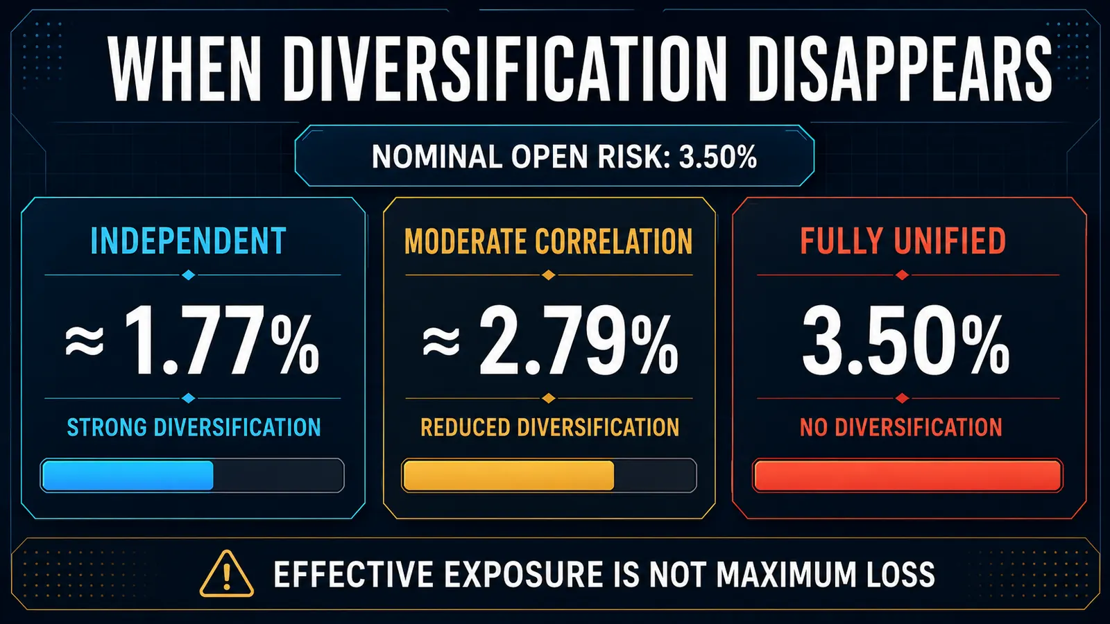
The comparison is the useful part. The portfolio is materially closer to a single concentrated bet than to four independent risks. The 2.79% estimate should not be presented as the maximum possible loss, nor should it be used to justify adding more trades simply because it is below the 3.50% nominal sum. The hard loss budget and the factor-concentration cap still apply.
What a risk engineer sees: the third or fourth trade is not evaluated in isolation. It is evaluated as an addition to an existing dollar cluster. Possible decisions include reducing its size, rejecting it, replacing it with a genuinely different exposure, sequencing entry until earlier risk is resolved, or accepting it only under a specifically authorized cluster budget.
Why Historical Correlation Is Not Enough
Correlation is an estimate, not a physical constant. Five weaknesses require explicit controls:
| Weakness | Risk | Control |
|---|---|---|
| Window dependence | Short windows are noisy; long windows can dilute the current regime. | Compare fast and slow windows; disagreement means uncertainty. |
| Timeframe/session mismatch | Daily relationships may not describe a ninety-minute London trade. | Match estimates to holding horizon and execution window. |
| Direction blindness | Raw price correlation ignores the chosen long and short directions. | Use signed trade returns or strategy P&L. |
| Regime instability | Central-bank paths, funding stress, or risk appetite can reverse relationships. | Combine rolling estimates with structural factor mapping. |
| Tail convergence | Modest normal correlation can rise sharply during repricing and thin liquidity. | Stress correlations, slippage, and spread assumptions. |
A Practical Correlation-Risk Pool Architecture
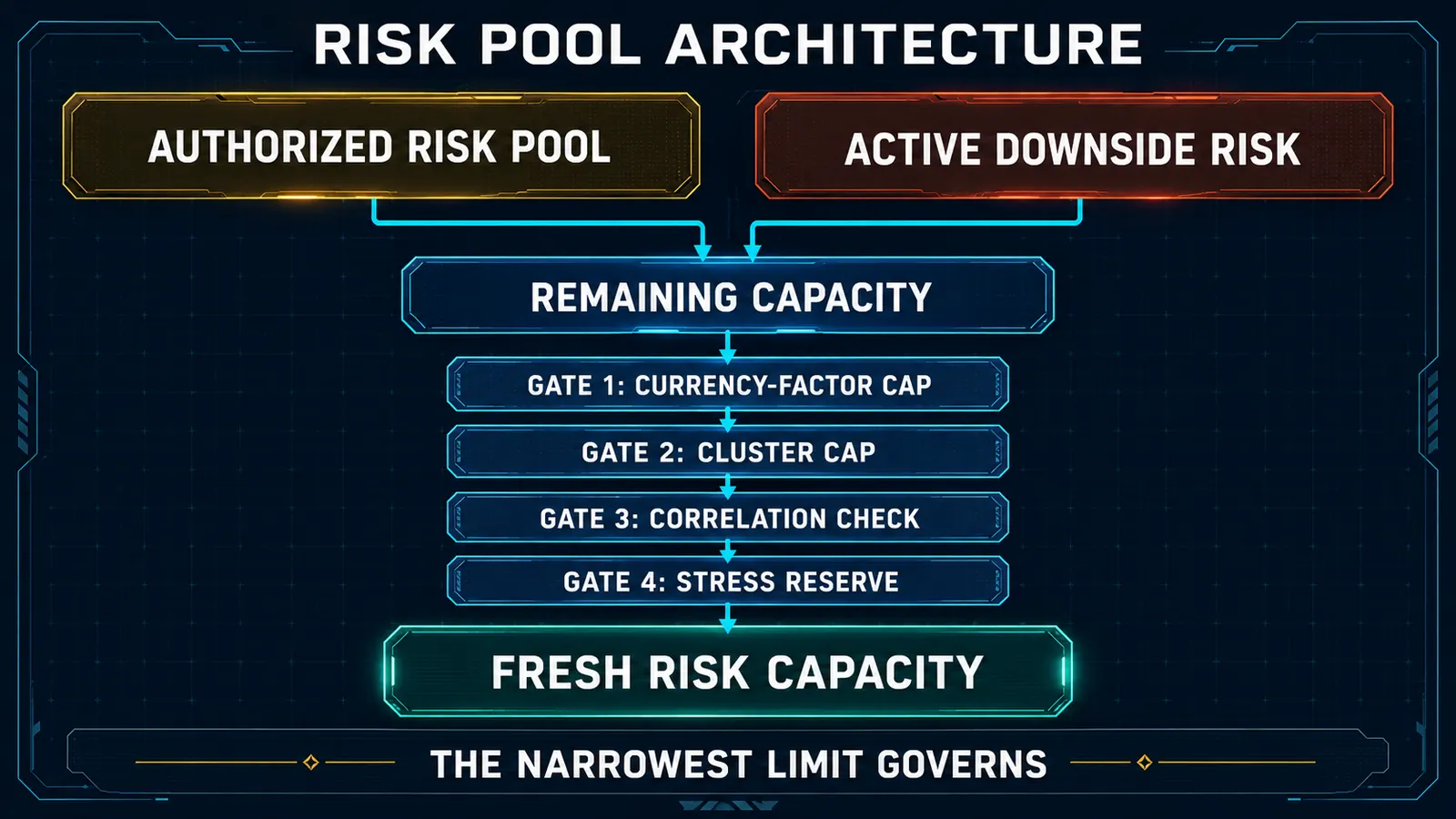
A risk pool is a finite amount of loss-bearing capacity authorized for a cycle, session, day, or portfolio state. It is not a target that must be fully deployed. Its purpose is to prevent independent trade decisions from collectively violating portfolio-level limits.
| Control layer | Question answered | Example rule |
|---|---|---|
| 1. Hard nominal-risk cap | What is the maximum planned stop risk currently open? | Total active downside risk cannot exceed the authorized pool. |
| 2. Currency-factor cap | How much risk depends on one currency direction? | Cap total short-USD or long-JPY risk inside the broader pool. |
| 3. Strategy/cluster cap | How much risk shares one thesis, setup family, or catalyst? | Limit one breakout cluster even across different symbols. |
| 4. Correlation-adjusted cap | How much diversification benefit survives after co-movement? | Reject additions that push effective exposure above tolerance. |
| 5. Marginal-addition test | What does the next trade add? | Size or reject based on incremental portfolio risk, not standalone risk. |
| 6. Stress overlay | What happens if correlations converge and fills worsen? | Use stressed coefficients and a slippage reserve around major events. |
The pool must compress when exposure carries forward
If open positions remain active into the next decision cycle, they have already consumed risk capacity. Fresh risk should be calculated from what remains, not from the original pool. This is smart-capacity logic: active downside risk is subtracted before new positions are sized.
Fresh capacity = max(0, authorized pool − active downside risk − reserves)
Reserves may include slippage allowance, event risk, fee drag, or a deliberate safety buffer. The key principle is non-negotiable: open risk compresses new deployment. Floating profit should not be treated as restored capacity unless the downside has genuinely been secured and the operating rules recognize the new stop state.
Illustrative limits — not universal defaults
A portfolio might authorize a 2.50% cycle pool, a 1.50% cap on any one currency direction, and a 2.00% cap on any one macro cluster. Those values are examples, not recommendations. Correct thresholds depend on strategy expectancy, stop behavior, gap exposure, trade frequency, drawdown tolerance, correlation stability, and Monte Carlo evidence.
The architecture matters more than the sample numbers. There should be a broad pool, narrower concentration limits inside it, and a rule that the narrowest applicable limit governs. If a new trade fits the total pool but violates the short-USD factor cap, it does not fit the portfolio.
The Pre-Trade Correlation Workflow
The workflow should be short enough to operate before execution but rigorous enough to block hidden concentration. A practical sequence is:
- Record current active downside risk by open position. Recalculate from current price and current protective stops; do not reuse stale initial-risk figures.
- Translate every open trade and the candidate trade into signed currency legs and broader factors such as USD direction, risk-on/risk-off, carry, commodity sensitivity, or regional exposure.
- Group positions into economic clusters. If several trades need the same macro move, treat them as a cluster even if their chart patterns differ.
- Check the hard portfolio pool and every relevant sub-cap: currency, strategy, catalyst, session, and cluster.
- Review fast-window, slow-window, and stressed correlation assumptions. Large disagreement should increase conservatism.
- Measure the candidate trade's marginal addition. Compare portfolio exposure before and after the trade.
- Choose the action: accept, reduce, delay, substitute, hedge, or reject. The setup's quality does not grant permission to bypass the risk architecture.
- Log the decision and the reason. Correlation overrides should be visible later in performance attribution and compliance review.
Decision actions are more useful than correlation labels
A dashboard that only colors correlation red or green is decorative. A risk system should issue an action:
- Accept when exposure is distinct and all limits hold; reduce when marginal contribution is excessive.
- Sequence entry until correlated risk clears, or substitute a less crowded exposure.
- Hedge only when basis, cost, and stress behavior are understood; otherwise reject the trade.
Common Failure Modes
| Failure mode | Why it fails | Engineering correction |
|---|---|---|
| Counting symbols | Different tickers can share the same currency or macro factor. | Map signed currency legs and economic clusters. |
| Using one correlation window | The estimate may be stale, noisy, or mismatched to the holding horizon. | Use fast, slow, and stressed views. |
| Ignoring trade direction | Raw negative correlation can become positive P&L dependence after long/short signs are applied. | Correlate signed trade returns or strategy P&L. |
| Treating low correlation as permission | Low historical correlation does not erase nominal stop risk or tail dependence. | Keep hard caps and stress overlays. |
| Sizing each trade independently | Every trade looks acceptable alone while the group violates the portfolio budget. | Run a marginal-addition test before entry. |
| Using floating profit as free capacity | Open profit can reverse; it is not the same as realized or protected capital. | Measure active downside from current stop state. |
| Hedging by label | An opposite-looking pair may introduce basis risk, new factors, and additional costs. | Test hedge behavior, cost, and stress stability. |
| Overengineering precision | Unstable inputs create a sophisticated-looking but fragile answer. | Use bands, conservative assumptions, and explicit uncertainty. |
Correlation Risk Is Also Behavioral Risk

Hidden concentration is often psychological as well as statistical. Several related charts can feel like independent confirmation even when they repeat one macro story. A risk pool closes that loophole by forcing conviction to compete for finite capacity rather than allowing repeated conviction to manufacture capacity.
Setup confidence may influence trade selection. It should not expand the portfolio's authorized risk pool. When several high-quality setups share one factor, the correct response is allocation — not accumulation.
What to Track After the Trades Close
Review decisions as clusters, not only as individual trades. Preserve enough journal data to reconstruct the portfolio at entry:
- signed factor tags, cluster identifier, and active risk before entry;
- remaining pool capacity and the candidate's marginal contribution;
- normal and stressed correlation bands plus any override reason;
- cluster P&L, simultaneous drawdown, loss clustering, and execution costs;
- whether apparent diversification survived in live conditions.